Power law extrapolation

(Warning: Just a toy model / very crude extrapolation, with no connection to reality.)

Background: https://twitter.com/svat/status/1814587528986419633

As of this revision, the article said:

wide use of Microsoft Windows and CrowdStrike software by large and global corporations in many business sectors. At the time of the incident, CrowdStrike said it had more than 24,000 customers, including nearly 60% of Fortune 500 companies and more than half of the Fortune 1,000.

Just as a toy mathematical model, can we, from these numbers and some power-law assumption, get some estimate of what fraction of organizations were affected, as a function of their size/rank — some number that would vary from 0.6 for “Fortune 500 companies”, down to 0 for home users/small companies (not using Crowdstrike)?

Well sure, it’s possible to draw a power law curve through two points :-)

(Unjustified) Assumptions:

• Every company has a distinct rank 1, 2, 3, ….
• For company with rank $k$, there is an associated number $p_k$, where $0\le p_k\le 1$.
• The sum of $p_k$ for $k\le 500$ is $0.6\times 500=300$. (This is treating “nearly 60% of Fortune 500 companies” as ”exactly 300 of the top 500 companies”.)
• The sum of $p_k$ for $k\le 1000$ is $0.5\times 1000=500$. (This is treating ”more than half of the Fortune 1000” as ”exactly 500 of the top 1000 companies”.)
• $p_k$ is a decreasing/non-increasing function of $k$, that moreover varies as a power-law: $p_k=c{k}^{-\alpha }$ for some constants $c$ and $\alpha$.

With these assumptions, we can work out the values of the constants $c$ and $\alpha$ from the two data points. Let $S_n=\sum _{k=1}^n{p}_k$. Then

$$\begin{array}{rl}{S}_{500}& =c\sum _{k=1}^{500}{k}^{-\alpha }=300\\ S_{1000}& =c\sum _{k=1}^{1000}{k}^{-\alpha }=500\end{array}$$

By dividing, we can calculate the value of $\alpha$ numerically: it is the value such that, if we define

$$f(\alpha )=\frac{\sum _{k=1}^{500}{k}^{-\alpha }}{\sum _{k=1}^{1000}{k}^{-\alpha }},$$ then $f(\alpha )=3/5$.

(More standard here may be the continuous approximation, or something formal with Hurwitz zeta function or whatever. But we can just do things numerically…)

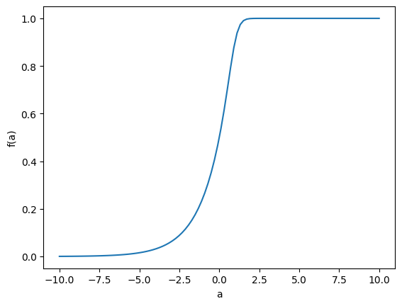
This is what $f$ looks like as a function of $\alpha$:

# prompt: Plot f as a function of a, from a = -10 to a = 10
import matplotlib.pyplot as plt
import numpy as np

x = np.linspace(-10, 10, 100)
y = [f(a) for a in x]

plt.plot(x, y)
plt.xlabel('a')
plt.ylabel('f(a)')
plt.show()

So finding $\alpha$ numerically:

lo = -10.0
hi = 10.0
eps = 1e-8
while hi - lo > eps:
  mid = (lo + hi) / 2
  if f(mid) < 0.6: lo = mid
  else: hi = mid
print(lo, hi)
# 0.2662351727485657 0.2662351820617914

gives $\alpha =0.266235$, after which we can plug back to get $c$:

a = 0.2662351789580996
print(300 / s(a, 500), 500 / s(a, 1000))
# 2.3161288835449767 2.3161288835449767

So we have our power-law distribution: $p_k=c{k}^{-\alpha }$ with $c=2.3161$ and $\alpha =0.2662$.

We can further truncate this to have total $24000$:

def p(k): return 2.3161288835449767 * k**-0.2662351789580996
s = 0
n = 0
while s < 24000:
  n += 1
  s += p(n)
print(n, s)
# 194633 24000.062311828504

This gives an updated function:

$$p_k=\{\begin{array}{ll}c{k}^{-\alpha }& \text{for }k\le 194633\\ 0& \text{for }k>194633\end{array}$$

(The sharp cut-off from $p_k\approx 0.09$ to $p_k=0$ shows that this toy power-law model is probably not a good reflection of reality, in case there was any belief left… but whatever.)

Let’s make it an interactive tool (used Claude): change the value of $k$ below (the “rank” of your company) to see corresponding value $p_k$, or vice-versa:

Edit: The same thing as a plot, again thanks to Claude:

And when viewed as a plot it shows why the model is nonsense, as it gives $p_k$ values greater than $1$ for small $k$.